
Graph neural networks
Introduction
Graph Neural Networks (GNNs) are neural network architectures that learn on graph-structured data. In recent years, GNN’s have rapidly improved in terms of ease-of-implementation and performance, and more success stories are being reported. In this post, we will briefly introduce these networks, their development, and the features that have led to their success.
We will dive deeper into three use-cases, citation networks, and drug discovery, using the package Deep graph library (DGL), and e-commerce using Pytorch geometric.
For a more thorough introduction to the mathematics of GNN’s, please have a look at my review paper (link).
Graph neural networks and their development
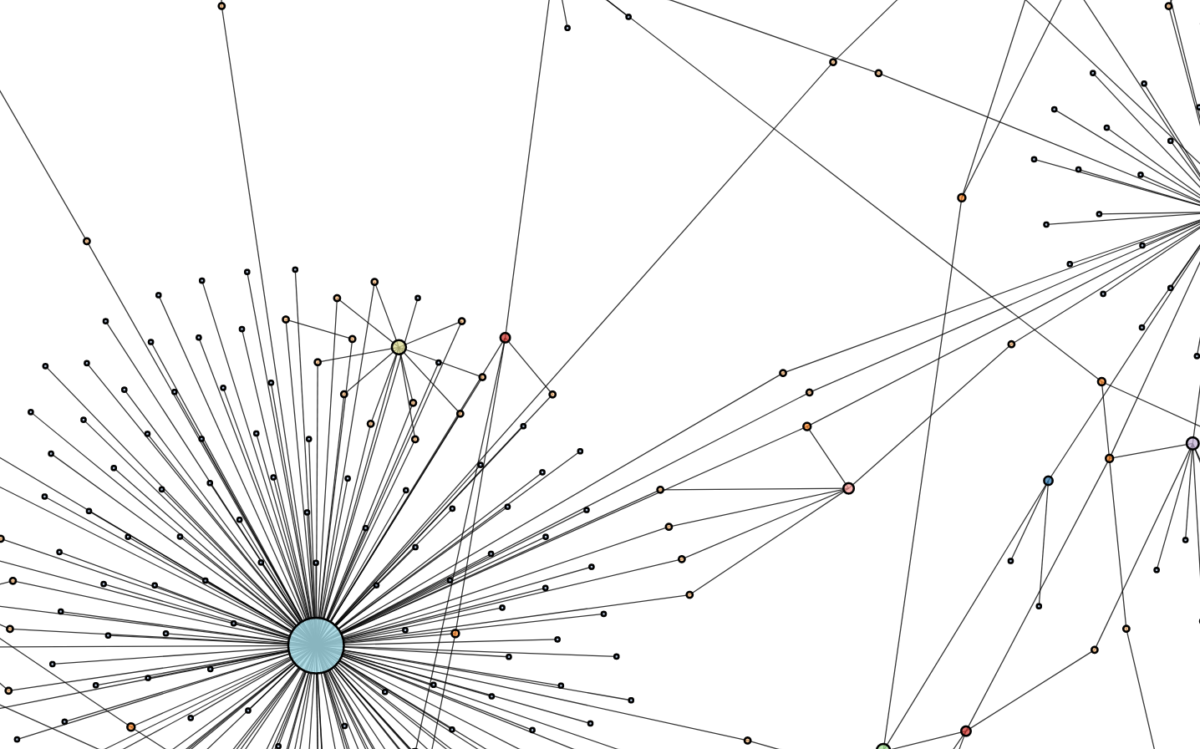
Graphs, commonly referred to as networks, are ubiquitous structures as a wide range of domains employ them to capture relationships (edges) between different entities (nodes). For example, in e-commerce, the network of items and users is modeled as a graph to predict new links representing a purchase or exploit interactions between users and products to produce high-quality recommendations. In chemistry, molecules are modeled as graphs, with atoms as nodes and edges as their bonds, to predict their bioactivity for drug discovery. Thus, as graphs are the founding structure in various systems, providing efficient and reliable algorithms to model graph networks is of great importance.
Graph Neural Networks (GNNs) have emerged as a generalization of neural networks that learn on graph-structured data by exploiting and utilizing the relationship between data points to produce an output. These architectures aim to solve tasks such as node representation, link prediction, and graph classification. Contrary to the euclidean space, operations that we take for granted, such as convolution, becomes increasingly difficult in the non-euclidean setting due to the lack of grid structure. Furthermore, the basic assumption that all data points are independent no longer holds as all data points are related to each other by edges.
Due to ambitious efforts of generalizing definitions and operations of traditional neural networks to graph settings, the field of GNNs has expanded explosively with novel architectures and has been introduced to a broader range of applications. Today GNNs can be divided into multiple categories: Graph Convolutional Neural Networks (GCNs), Recurrent Graph Neural Networks (RGNNs), Graph Attention Networks (GANs), Graph Auto-encoders (GAEs), Graph Spatial-temporal Networks (GSTNs), and Graph Reinforcement Learning, all of which continue to grow with new methods and models.
One of the first models proposed within GNNs is RGNNs. They were originally proposed to extend Recursive Neural Networks, which also operate on graphs but require them to be directed and acyclic. RGNNs loosen this restriction by handling any type of graph. Even though these architectures were proposed already back in 2009, it took some time before GNNs gained attention. One of the breakthroughs in this area was when GCNNs were introduced, especially when spatial-based GCNNs were proposed. To perform convolution on a graph, the convolution operation had to be generalized to the non-Euclidean setting. This was done by using the Convolutional theorem as a definition and performing the convolution in the Fourier domain. By using a spectral representation of the filters, this approach was named ’the spectral-based approach.’ However, the spectral-based approach suffered from several limitations. It could not generalize to new, unseen data, and the operations required were costly; for graphs larger than a few thousand nodes, the computations were inefficient. Thus several simplifications had to be made. Hammond et al. showed that it is possible to approximate the convolution between two functions on the graph’s nodes by low-ordered truncated Chebyshev polynomials. By further simplifications, Kipf et al. could perform the convolution by only including information from the neighboring nodes and thus only using the graph’s spatial information. Therefore, this was called the spatial-based approach.
The spatial-based approach was further generalized to the message passing scheme commonly used for all GNNs – the models are distinguished by choice of the aggregate– and combine– functions. Nodes are sending their state and features, messages, to the neighboring nodes along the edges. The kth layer of an arbitrary GNN is given by
\bm{m}_i^{(k)} = aggregate^{(k)} \big( \big\{ \bm{h}_j^{(k-1)}: j \in \mathcal{N}(i) \big\} \big), \newline \bm{h}_i^{(k)} = combine^{(k)}\big(\bm{h}_i^{(k-1)}, \bm{m}_i^{(k)} \big) \newline\text{where }\bm{h}_j^{(k)} \text{is the feature vector of node } j \newline \text{ at the }\text{k}^{th} \text{layer},
\text{and } \mathcal{N}(i) \newline \text{ represents the neighbours of } i. Application of GNN’s
In this part, we go through some applications for GNN’s. For more examples, consult https://arxiv.org/pdf/1812.08434.pdf, which lists more than twenty in NLP, computer vision, medicine, chemistry, and information processing).
There are multiple ways of implementing graph neural networks; some of the most frequently used packages are PyTorch geometric, Deep graph library (DGL), and Spektral. PyTorch geometric use PyTorch as backend, and DGL supports both PyTorch and MxNet while Spektral uses Tensorflow as backend. In our examples, we will use DGL and PyTorch-geometric.
Citation networks
Citation recommendation systems play an important role in research as it helps researchers to find and cite all relevant papers. Thus, being able to categorize papers into different research fields could help in this task. To demonstrate how we could use GNNs to solve this task, we will use the Cora dataset and the DGL module, and showcase a simple implementation of an off-the-shelf Graph Attention Network. The model can then be used to predict probable citations given an article
We start by downloading the data by using DGLs API and extracting node features and labels, as well as the masks for dividing the dataset into a train, test, and validation dataset. The node features of the dataset are 1433-sized 0/1 vectors corresponding to the absence/presence of a word from a dictionary. The task is to classify each node (article) into one of seven classes (fields).
# Downlod the cora dataset
dataset = CoraGraphDataset()
g = dataset[0]
# get node feature
features = g.ndata['feat']
# divide dataset
train_mask = g.ndata['train_mask']
val_mask = g.ndata['val_mask']
test_mask = g.ndata['test_mask']
#get labels labels = g.ndata['label']
We build a 2-layer GAT-model using dgls pre-build GCN-module and define accuracy as our metric.
import dgl
from dgl.nn.pytorch.conv import GATConv
from dgl.data import CoraGraphDataset

import torch
import torch.nn as nn
import torch.nn.functional as F

class GAT(torch.nn.Module):
    def __init__(self, in_dim, hidden_dim, out_dim, num_heads):
        super(GAT, self).__init__()
        self.layer1 = GATConv(in_dim, hidden_dim, num_heads)
        self.layer2 = GATConv(hidden_dim * num_heads, out_dim, 1)

    def forward(self, g, h):
        h = self.layer1(g, h)
        h = h.view(-1, h.size(1) * h.size(2))
        h = F.elu(h)
        h = self.layer2(g, h)
        h = h.squeeze()
        return h
def accuracy(logits, labels):
    _, indices = torch.max(logits, dim=1)
    correct = torch.sum(indices == labels)
    return correct.item() * 1.0 / len(labels)


def evaluate(model, features, labels, mask):
    model.eval()
    with torch.no_grad():
        logits = model(features)
        return accuracy(logits[mask], labels[mask])
We initialize the model and train for 10 epochs.
net = GAT(in_dim=features.size()[1],
          hidden_dim=10,
          out_dim=7,
          num_heads=2)

# create optimizer and define loss function
optimizer = torch.optim.Adam(net.parameters(), lr=0.01, weight_decay=0.001)
loss_fcn = torch.nn.CrossEntropyLoss()

train_accuracy = []
val_accuracy = []
loss_list = []
for epoch in range(10):
    logits = net(g,features)
    loss = loss_fcn(logits[train_mask], labels[train_mask])
    loss_list.append(loss)

    optimizer.zero_grad()
    loss.backward()
    optimizer.step()

    train_acc = accuracy(logits[train_mask], labels[train_mask])
    train_accuracy.append(train_acc)

    val_acc = accuracy(logits[val_mask], labels[val_mask])
    val_accuracy.append(val_acc)

    print("epoch {:05d} | loss {:.4f} | train acc {:.4f} |"
          " val acc {:.4f} ".
          format(epoch, loss.item(), train_acc, val_acc))
As you can see, we can train it just like any other network in PyTorch. Here we train it for 10 epochs and we get a test accuracy of 0.74.
epoch 00000 | loss 1.9465 | train acc 0.1786 | val acc 0.1280
epoch 00001 | loss 1.9263 | train acc 0.6571 | val acc 0.4440
epoch 00002 | loss 1.9067 | train acc 0.9429 | val acc 0.6200
epoch 00003 | loss 1.8871 | train acc 0.9714 | val acc 0.6900
epoch 00004 | loss 1.8673 | train acc 0.9643 | val acc 0.7080
epoch 00005 | loss 1.8471 | train acc 0.9643 | val acc 0.7240
epoch 00006 | loss 1.8264 | train acc 0.9643 | val acc 0.7320
epoch 00007 | loss 1.8054 | train acc 0.9571 | val acc 0.7340
epoch 00008 | loss 1.7839 | train acc 0.9571 | val acc 0.7340
epoch 00009 | loss 1.7621 | train acc 0.9500 | val acc 0.7460
Recommender systems
One key application for GNNs is recommender systems.
This application addresses how many different customers have bought some products (or rate them, as in the Netflix dataset). The customers (usually referred to as users) interact with the products (usually referred to as items) to form an interaction matrix. These recommender systems can be constructed in many different ways; the most basic one is a collaborative filtering approach. The end goal is to predict the probability of a user buying an item (or predict the rating).
We will showcase a simple recommender system implemented in PyTorch geometrics, using the youchoose-dataset released in the Recsys challenge 2015. The dataset comes from a European retailer who tracked which sessions ended up with a purchase and which didn’t

The dataset consists of two files, yoochoose-clicks.dat, and yoochoose-buys.dat. The clicks-file contains all the sessions and which items the end-user has clicked on, while the buys-dataset contains which session leads to a purchase. An interesting part of this problem is actually not only the network but how to construct the dataset. We will treat each session as a graph, where each item in the session is a node. Instead of each graph having one target, the target for a graph is of the same size as the number of items in that graph, and if an item is bought within the session, the label corresponding to that item is set to 1. After the preprocessing, we load the data into the data loader.
from torch_geometric.data import DataLoader
batch_size= 512
train_loader = DataLoader(train_dataset, batch_size=batch_size)
val_loader = DataLoader(val_dataset, batch_size=batch_size)
test_loader = DataLoader(test_dataset, batch_size=batch_size)
The datasets are now ready for training. We create embeddings for the categories and item ids and build the model using the PyTorch geometric GCNConv-module. It is a straightforward model, only using one GCN-layer followed by a top-k pooling layer and 2 fully connected layers. A top-k pooling layer selects the k nodes that are given the highest score. If you are curious about these layers, you can read more about them here.
embed_dim = 128
from torch_geometric.nn import GraphConv, TopKPooling
from torch_geometric.nn import global_max_pool
import torch.nn.functional as F

class Net(torch.nn.Module):
    def __init__(self):
        super(Net, self).__init__()
        self.item_embedding = torch.nn.Embedding(
                 num_embeddings=num_items, embedding_dim=embed_dim)
        self.category_embedding = torch.nn.Embedding(
                 num_embeddings=num_categories, embedding_dim=embed_dim)

        self.conv = GraphConv(embed_dim * 2, 128)
        self.pool = TopKPooling(128, ratio=0.9)

        self.lin1 = torch.nn.Linear(128, 256)
        self.lin2 = torch.nn.Linear(256, 128)

        self.act1 = torch.nn.ReLU()
        self.act2 = torch.nn.ReLU()

    def forward(self, data):
        x, edge_index, batch = data.x, data.edge_index, data.batch

        item_id = x[:,:,0]
        category = x[:,:,1]


        emb_item = self.item_embedding(item_id).squeeze(1)
        emb_category = self.category_embedding(category).squeeze(1)

        x = torch.cat([emb_item, emb_category], dim=1)
        x = F.relu(self.conv(x, edge_index))
        x, edge_index, _, batch, _, _ = self.pool(x, edge_index, None, batch)
        x = global_max_pool(x, batch)

        x = self.lin1(x)
        x = self.act1(x)
        x = self.lin2(x)
        x = F.dropout(x, p=0.5, training=self.training)
        x = self.act2(x)

        outputs = []
        for i in range(x.size(0)):
            output = torch.matmul(emb_item[data.batch == i], x[i,:])

            outputs.append(output)

        x = torch.cat(outputs, dim=0)
        x = torch.sigmoid(x)

        return x
We train the network for 3 epochs and gain a training AUC of 0.64.
for epoch in range(3):
    loss = train()
    train_acc = evaluate(train_loader)
    val_acc = evaluate(val_loader)
    test_acc = evaluate(test_loader)
    print('epoch: {:03d}| loss: {:.5f} | train auc: {:.5f} | val auc: {:.5f} | test auc: {:.5f}'.
          format(epoch, loss, train_acc, val_acc, test_acc))
epoch: 000| loss: 0.59050 | train auc: 0.54846 | val auc: 0.52429 | test auc: 0.53870
epoch: 001| loss: 0.42529 | train auc: 0.60686 | val auc: 0.56317 | test auc: 0.57504
epoch: 002| loss: 0.37031 | train auc: 0.64619 | val auc: 0.57692 | test auc: 0.58595
This could of course be improved in a real-world application by, e.g., increasing the training time, tweaking the model architecture, and hyper-parameter optimization.
Drug discovery
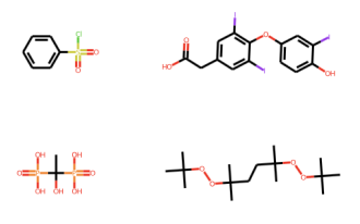
In computer-aided drug design, a crucial step is to assess the properties of new, complex molecules quickly. Molecules are quite intricate graphs, and small changes can significantly impact the molecule concerning some properties (toxicity, reactivity, polarization, etc.). Also, how the molecule interacts with other molecules (e.g., protein-protein interactions) is an area where GNN’s is well suited.
The area of drug discovery is quite wide in terms of which properties of the molecule one wish to investigate. As previously mentioned, these properties cograph-network could be toxicity, reactivity, polarization for example. In this use case, we will try to predict the toxicity of molecules using a convolutional neural network for graphs, implemented in PyTorch geometrics.
The dataset used is called “Toxicology of the 21st century” (Tox21). The dataset contains approximately 8k compounds, with 12 metrics used to measure toxicity. These include nuclear receptors (NR) and stress response pathways (SR). Each of these measurements results in a binary label.
All molecules in the dataset are encoded by a string representation of their 2D structure, called SMILES. Pytorch geometrics uses this representation to calculate features such as atomic number, chirality, change, and the number of radical electrons. The dataset is easily downloaded using Pytorch geometrics API.
from torch_geometric.datasets import MoleculeNet
tox21 = MoleculeNet(root=os.path.join(os.getcwd(), 'data'), name='Tox21')
As previously mentioned, toxicity is measured by 12 different metrics. This means that one molecule may be toxic based on several metrics and thus belong to several classes. Also, all the molecules might not be tested by all metrics which results in NaNs. Now, there are many ways to deal with data points belonging to several classes, but in the simple showcase, we change this problem from a multiclass problem to a binary one by classifying the compound as toxic if any of the metrics show toxicity. This will result in a binary label; toxic or not toxic. Furthermore, in this problem, we will simply disregard the missing values. Therefore we set the target as follows.
target_df = pd.DataFrame(tox21.data.y.numpy())
target = torch.tensor(np.where((test_df == 1).any(axis=1) == True, 1, 0))
The features provided by MoleculeNet is discrete and of type long, so we need to convert them to continuous embeddings, which is done by the following code snippet.
class AtomEncoder(torch.nn.Module):
    def __init__(self, hidden_channels):
        super(AtomEncoder, self).__init__()

        self.embeddings = torch.nn.ModuleList()

        for i in range(9):
            self.embeddings.append(torch.nn.Embedding(100, hidden_channels))

    def reset_parameters(self):
        for embedding in self.embeddings:
            embedding.reset_parameters()

    def forward(self, x):
        if x.dim() == 1:
            x = x.unsqueeze(1)

        out = 0
        for i in range(x.size(1)):
            out += self.embeddings[i](x[:, i])
        return out
This network can now be trained like the other two examples. This problem can also quite easily be solved using DGL, which has already trained a model for this dataset. Take a look at this example.
from dgllife.data import Tox21
from dgllife.model import load_pretrained
from dgllife.utils import smiles_to_bigraph, CanonicalAtomFeaturizer

dataset = Tox21(smiles_to_bigraph, CanonicalAtomFeaturizer())
model = load_pretrained('GCN_Tox21') # Pretrained model loaded
model.eval()

smiles, g, label, mask = dataset[0]
feats = g.ndata.pop('h')
label_pred = model(g, feats)
Wrapping up
This post provides an overview of graph neural networks and some practical applications. In short, Graph neural networks and all their kinds can provide a way to better represent and learn from non-traditional datasets. In some cases, it provides a superior approach compared to traditional methods. Although GNN’s can be somewhat cumbersome to wrap one’s head around, the non-euclidean nature’s implementation is not necessarily more tedious than a conventional neural net. It will be interesting to follow this branch of ML in the coming years!