- 33 min read
- Cross-industry
- Oct 2026
Reinforcement learning for small language models

Introduction
TLDR: We built two environments, trained Qwen3 models at 0.6B, 1.7B and 4B with GRPO in prime-rl, and measured how well small self-hosted models perform. On a narrow, well-scoped tool-use task (customer-email handling over an invoice database), GRPO takes a 0.6B model from 0.422 to 0.968 pass@1. On an open-ended multi-hop retrieval task, SFT on rejection-sampled teacher trajectories followed by GRPO lifts a 4B model from effectively zero to 0.335 pass@1. With a revised prompt and reward and more training data, it reaches 0.446, competitive with a prompted frontier model on the same harness, at a fraction of the per-question cost, and without any data leaving our own hardware.
Agentic systems are token-hungry, and running them on frontier models from the big providers gets expensive fast. Many of our clients are also uneasy about sending sensitive data to external model providers. A frontier model is built to handle anything you might ask it, but most production agents ask one thing, over and over, and you pay for that generality whether you need it or not. A natural way of addressing both concerns is to self-host smaller language models and tune them to your specific needs. The usual ways to do that tuning are prompt engineering and supervised fine-tuning on demonstrations. For agentic tasks there are often many different routes to the correct answer, and demonstrations force the model to imitate one of them rather than find its own route. When success is cheap to verify but good demonstrations are expensive, reinforcement learning (RL) is a natural fit.
We wanted to find out how close a small self-hosted model trained with RL gets to a frontier-lab model, and how much the training recipe matters. Along the way, we also wanted to collect practical answers for anyone doing this themselves: how much data, compute and time it took us, and what difference the reward design made.
The experiments cover two environments, three model sizes, three training recipes and a final tuned configuration at 4B. They show which recipe works at which model size, what a self-hosted model costs per question compared with an API model, and where the models still fail. We start with a short introduction to RL for language models, from the policy gradient theorem to GRPO, and then look at prime-rl, the framework we used, and how its design follows from that theory. Readers already familiar with RL can skip ahead to the second section, or straight to the experiments.
RL for language models
Classical RL is formulated over a Markov decision process , made up of a state space , an action space , transition dynamics , a reward function and a discount factor . A standard example is the grid world, where the state is the cell , the actions are , and the transitions are given by the rules of the world.
For a language model the mapping is:
- State : the text so far: the prompt plus the partially generated response.
- Action : the next token to generate (the action space is the model's vocabulary).
- Trajectory : a full rollout.
- Transitions: deterministic concatenation, .
Rewards are typically sparse and terminal: for all , and is whatever the verifier says. With the return is simply .
When the model only generates text, everything after the prompt is its own output, and no reward arrives until the end. The "MDP" then degenerates into something much closer to a contextual bandit: the model picks one long action, a completion, and is scored once. The exception is tool use. When the model emits a tool call, the environment injects tokens the model did not choose, and we are back to the MDP framing. Both environments we discuss below involve tool use.
Policy optimization and the policy gradient theorem
With the setup in place, the question is how to update the model so that high-reward trajectories become more likely. Let be the policy, our LLM parameterized by , and the distribution over trajectories induced by rolling it out in the environment. The objective is to maximize the expected return:
Computing this directly is intractable, because the sum runs over every possible token sequence, an astronomical number of combinations. The policy gradient theorem gives us a way out. Using the identity , we get:
The final equality follows because , and neither the initial-state distribution nor the transition dynamics depend on , so their gradients vanish.
This property makes RL practical for LLMs. The gradient depends only on the policy, not on the environment, so we never need to differentiate through the tool calls, the database or the search index. All we need is to sample from the environment and score the result. That is the sense in which RL is "model-free," and it is why an RL environment can be an arbitrary blob of Python.
The expectation is still not something we can compute, but unlike the original sum it is now over trajectories we can sample. Rolling out the policy times and averaging gives
which is an unbiased estimator of : averaged over many batches, it equals the true gradient. This estimator, and the algorithm that plugs it into stochastic gradient ascent, is REINFORCE [Williams, 1992]. Unfortunately, in its raw form it is nearly useless, because the variance is enormous.
Cutting variance: baselines and the critic
The problem is that is an absolute quantity. Suppose three rollouts of the same prompt score . All three get pushed up, the first most strongly. Now suppose they instead score : the same average, but no spread. There is nothing to learn, since no completion is preferable to any other, yet REINFORCE still returns a large gradient on every sample.
The policy is a normalized distribution over completions, so training can only move probability mass between them. A term shared by all three says nothing about which way to move it. We can see this directly from normalization. Since for every ,
and is exactly the per-sample gradient above. So the shared multiplies a quantity whose mean is zero and contributes nothing in expectation. But we never take that expectation. We average three samples, and over three samples the term does not cancel; instead, it scales up whatever noise those gradient terms carry. The is the entire usable signal, riding on a term fifty times its size.
The fix is to subtract a baseline that does not depend on the action. For the same reason as before, , so any such baseline leaves the estimator unbiased, and a well-chosen one reduces its variance. Replacing the return with an advantage
gives . The baseline depends on the state, so the same trajectory return is scored differently at different points in the rollout. The variance-minimizing choice is (approximately) the value function , the expected verifier score given the text generated so far, which we do not have, so in PPO-style methods we learn it: a second network , the critic, trained alongside the policy to predict the observed returns.
The advantage can then be understood as "how much better was this action than what we expected from this state", which is the quantity we actually want to reinforce.
Keeping updates stable: PPO
Vanilla policy gradients are on-policy: the data must come from the current policy. As soon as we make a single parameter update based on a rollout, that rollout is technically off-policy. Reusing a batch of rollouts for many gradient steps is still far more sample-efficient. The problem is that each step makes the data staler, and a large update on stale data can destroy the policy outright.
The standard correction is importance sampling: to estimate an expectation under using samples drawn from , reweight each sample by how much more or less likely it is under the new policy,
so that . A token the new policy now favors is up-weighted, one it has moved away from is down-weighted, and the stale batch is made to stand in for fresh samples. The catch is variance: the correction is only trustworthy while the two policies are close, and a large ratio on a single token is enough to wreck an update.
PPO (Proximal Policy Optimization) [Schulman et al., 2017] keeps the ratio but stops trusting it once it moves far from 1, that is, once the new policy has drifted from the one that generated the data:
The clip range (typically 0.2) defines a trust region: once the new policy has moved far enough from the generating policy on a given token, the objective flattens and that token stops contributing to the gradient.
The cost of a critic and the motivation behind GRPO
PPO trains a critic alongside the policy, typically initialized from a model of comparable size. Because the critic is trained rather than frozen, it carries the same per-parameter cost as the policy in weights, gradients and optimizer state, roughly doubling the memory footprint, not counting activations.
So: can we get a baseline without a critic? GRPO (Group Relative Policy Optimization) [Shao et al., 2024] takes a different approach: sample a group of rollouts for the same prompt (e.g. ) and use the group's own statistics as the baseline:
where is the verifier reward of rollout . The advantage is a single scalar per rollout, applied to every token in it. Plugging this advantage into the PPO objective, with a KL penalty against a frozen reference policy, gives:
where is the -th rollout. We drop the critic and pay for it with rollouts per prompt instead of one. For LLMs that is usually worth it: rollouts parallelize across GPUs and can be pushed to a separate inference engine, while a second trainable network has to sit in the training GPUs' memory alongside the policy.
If all rollouts in a group score identically, say all 0 on a question the model cannot solve or all 1 on one it always solves, every advantage is zero and the group contributes no gradient. Task difficulty has to sit in the band where the model sometimes succeeds, and for small models, keeping it there is the central practical challenge. Dynamic sampling, curriculum learning and online difficulty filtering are common ways to handle it.
What we want from an RL framework
The section above explains a fair amount about why libraries like prime-rl and verl are built the way they are. We have the following:
- Generation dominates compute. With rollouts per prompt and multi-turn tool use, the vast majority of wall-clock time is inference. That calls for a fast, separate inference engine.
- Training and inference should be decoupled and fully async. Neither side should idle waiting for the other, which means the two run as separate processes rather than alternating in one.
- The generating policy is not the trainer's current policy. Once the two run asynchronously, they drift, and the framework has to deal with the gap. The upside is that a batch of rollouts stays usable for more than a single update.
We use prime-rl for the experiments because it is built around exactly these three points. In Prime Intellect's own words, it is "a framework for large-scale reinforcement learning designed to be easy to use and hackable, yet capable of scaling to 1000+ GPUs." It is split into two repositories:
- prime-rl: the training infrastructure.
- verifiers: the environment and reward library, where an environment is just a self-contained Python module.
Most of the practices the GRPO literature has converged on are already in prime-rl, either enabled by default or easy to turn on. At the time of our runs, that included:
- Dynamic sampling, which drops groups whose rollouts all score identically, since they carry no gradient, and over-provisions rollouts so the batch can be refilled without stalling the step [Yu et al., 2025].
- Rollout filters for gibberish and repetition collapse, plus plugin hooks for your own advantage and filtering criteria.
- Difficulty-aware sampling that keeps prompts in the band where groups still have variance.
- Corrected loss normalization, removing the length and standard-deviation biases in the original GRPO objective [Liu et al., 2025, Dr. GRPO].
- Importance-ratio correction with two-sided clipping, which compensates for the off-policy gap from point 3 instead of just tolerating it [Prime Intellect, 2025].
- Loss masking of environment tokens, so tool returns condition the policy without the policy being trained to produce them [Jin et al., 2025]. Recent work such as ECHO (also available in prime-rl) deliberately trains on these tokens instead, adding an auxiliary next-token loss on tool outputs so the policy learns a world model of its environment [Shrivastava et al., 2026].
- SFT and distillation modes in the same framework, used by Recipe 2 below.
prime-rl moves quickly, so treat this as a snapshot rather than a complete feature list.
Experiments
Answering the questions from the introduction requires environments where success is cheap to verify, more than one model size, and recipes that differ in one component at a time.
We built two environments. The first is a narrow, well-scoped tool-use task of the kind a client would actually deploy. The second is open-ended multi-hop retrieval, where we expected the small models to struggle. On the second, we trained Qwen3 at 0.6B, 1.7B and 4B under three recipes, then tuned the best 4B setup further and compared it against a prompted frontier model on the same harness.
All training runs on two NVIDIA RTX A6000s on our company server, and in all experiments we train LoRA adapters rather than full models. We did not tune hyperparameters per recipe. Each run took long enough that every recipe was trained once with the same settings and evaluated once, and no model was retrained based on its evaluation results. The exceptions are the prompt changes and final runs in the Haiku section, which were informed by the earlier results, as described there.
Environment 1: Supplier invoices, a narrow production-shaped task
This environment simulates a customer-service agent handling incoming email about subscriptions, suppliers and invoices. The model reads an email, works out what is being asked, calls one or more tools against a synthetic SQLite database, and replies in free text.
We define three tools, each wrapping an underlying SQL query:
GetOrderBySubscription(sub_no): looks up a subscription number and returns its order rows, newest delivery period first.SearchSupplier(name?, iban?, bankgiro?, postgiro?, vat_number?): searches the supplier records with bank details. Identifier matching ignores spaces and dashes, and all provided parameters must match.LookupOrderRows(supplier_id, period_start?, period_end?, product_name?, subscriber_name?): searches a supplier's order rows with a period-overlap filter and partial matching on product and subscriber.
LookupOrderRows takes a supplier_id UUID, which is only obtainable from SearchSupplier. Harder tasks therefore require chaining: resolve the supplier first, carry its id forward, then query its order rows.
Database. The schema is a SQLite translation of parts of a client's production tables, trimmed to the columns that matter for matching: invoices and invoice rows join to order rows, which join to products and their suppliers on one side and to departments and their parent corporations on the other. The contents are synthetic. A single procedural pass with a fixed seed populates the database and samples the task scenarios together, which makes the gold answer correct by construction: each task carries a gold SQL query, and the answer is whatever that query returns against the shipped database. It is small (149 suppliers, 597 products, 96 client organizations and 1,329 order rows across 600 invoices), so every lookup a task needs is cheap.
Dataset. We generated 2,000 tasks, each a {question, gold_values} pair. The generation pipeline is hybrid: the procedural pass above fixes the facts of each scenario, including all customer, supplier and organization names, then Claude Sonnet writes the email text, and a validation pass checks that the required facts are present and the gold answer does not leak into the email. All tasks are email-shaped, 50/50 Swedish/English, roughly 85% from client-org staff and 15% from end customers, spanning five question types. The three easy types (~58% of tasks) are answerable with a single tool call. The medium and hard types (~42%) require at least two, since the supplier must be resolved by name or by bank identifier before its order rows can be looked up. Tasks 0–1799 are used for training and 1800–1999 for validation, split so that no supplier or organization in the validation set appears in training.
Example of a generated task:
{
	"question": "Subject: Details for subscription 67484\n\nHi,\n\nWe're reviewing our subscription portfolio and need to confirm which publication subscription 67484 covers, and which department at our
	organisation holds it. Could you please provide that information?\n\nRegards,\nPer Falk\nOffice Manager, Strängnäs Universitet",
	"gold_values": ["Nordic Mining Quarterly", "STRÄNGNÄS FORSKNINGSENHET"],
	"info": {
	  "scenario_id": 68,
	  "qtype": "sub_product_dept",
	  "register": "client_org",
	  "language": "en",
	  "difficulty": "easy"
		}
	}
This is an easy task, because a single call to GetOrderBySubscription(67484) returns both the product and the department.
We score the output by simply checking what fraction of gold values are present in the final reply, matched on word boundaries so that e.g. active does not match inactive. A task counts as passed when all of the gold values are present.
Before training, we ran the base model, Qwen3-0.6B, on the validation split to see how well it performs out of the box. Besides giving us a baseline, this indicates whether the environment is suitable for GRPO at all: if it is too hard, the model will never produce a correct rollout, and there will be no training signal to learn from.
| Model | pass@1 | pass@2 | avg tool calls |
|---|---|---|---|
| Qwen3-0.6B (base) | 0.422 | 0.532 | 1.265 |
This is a workable starting point. The model already solves a fair share of tasks but is nowhere near perfect, so most groups should contain both successes and failures rather than collapsing to a uniform score.
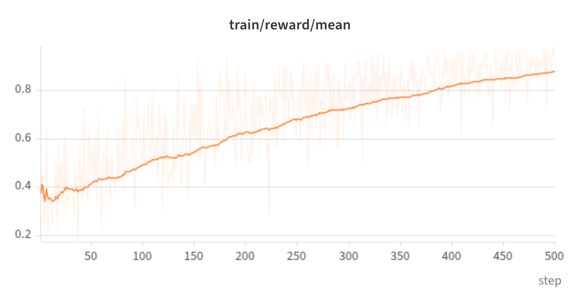
We trained Qwen3-0.6B with GRPO for 500 steps. Each prompt gets a group of rollouts, and each step trains on 32 rollouts, so 4 distinct tasks per update. Over 500 steps that is 2,000 group draws against 1,800 training tasks, roughly a single pass over the split. Reward is outcome-only, the fraction of gold values present in the final reply, so the policy is free to route tool calls however it likes; wrong routing simply fails to produce the answer.
As described in the prime-rl section, zero-variance groups are dropped before they take up batch slots, and gibberish and repetition-collapsed rollouts are filtered out. Here, 64 rollouts are kept in flight against the 32 needed per step, so discarded groups can be refilled without stalling training. The plot below shows the reward increasing during training (smoothed with a time-weighted EMA):
We evaluated on the same validation split as before, with the baseline repeated for comparison:
| Model | pass@1 | pass@2 | avg tool calls |
|---|---|---|---|
| Qwen3-0.6B (base) | 0.422 | 0.532 | 1.265 |
| Qwen3-0.6B (GRPO) | 0.968 | 0.988 | 1.588 |
The mix of task difficulties implies a floor of about 1.4 tool calls per task (58% need one call, 42% need at least two). The base model sits below it at 1.3, answering after a single call and failing the tasks that need two, and training pushes it to 1.6. Outcome-only reward was enough to teach the routing, without any direct supervision of it.
At a pass@1 of 0.968, the environment is close to exhausted. Almost every group now scores uniformly and contributes no gradient, which is the all-ones case from earlier, and there is little left for further training to extract.
The environment lacks the usual sources of difficulty in agentic tasks. The tool surface is small and fixed, no task needs more than one hop of indirection, and correctness is a string match. A 0.6B model saturating it in a few hours on two A6000s is about what you would expect. The second environment is harder on all three counts, letting us test how much model size and training recipe matter.
Environment 2: Agentic multi-hop retrieval
The second environment simulates agentic retrieval: the agent receives an information request that can only be answered from internal documentation, using a search tool over a corpus of documents. The questions are multi-hop, so answering one takes several searches. The model has to decide what to search for next based on what earlier results returned, and then reason over everything it found to produce an answer.
The dataset
We built a custom dataset based on MuSiQue [Trivedi et al., 2022] (HF dgslibisey/MuSiQue), using its validation split of 2,417 answerable multi-hop questions. MuSiQue is built bottom-up by mining single-hop questions from SQuAD, Natural Questions, T-REx, Zero-shot RE and MLQA, and chaining 2 to 4 of them so that one hop's answer is an entity in the next hop's question ("the actor of movie X is Y; Y was born in Z; so Z is the answer"). In the original setting, each question is paired with ~20 candidate paragraphs that are all supplied in the prompt, so retrieval is not part of the task, only reasoning.
Since we wanted to train retrieval, we pooled the paragraphs from all questions into a single deduplicated corpus and indexed it once with BM25, giving 21,100 passages and one shared search index. This change has three effects:
- The hops become retrieval-sequential. Hop 2's paragraph cannot be retrieved until hop 1 reveals the bridge entity, because that entity does not appear in the original question. A single BM25 query over the question typically reaches only the first hop. That makes it a genuine agentic search problem rather than single-shot RAG over a larger corpus.
- The distractors get stronger for free. MuSiQue's original 20-paragraph bundles were adversarially populated with topically adjacent paragraphs, and pooling them yields a corpus that is lexically dense around every gold entity. The corpus is full of look-alikes by design.
- The scale is realistic. At ~21k passages, the corpus is comparable in size to a mid-sized company's internal documentation: small enough for a single lexical index to be practical, but large enough that retrieval is non-trivial.
Example question from the dataset:
{
  "question": "What guarantees fundamental rights in the birth country of The Mystic Masseur's producer?",
  "answer": "Part III (Article 12 to 35) of Constitution of India",
  "info": {
    "id": "4hop1__783955_415728_50519_64447",
    "hop_count": 4,
    "answer_aliases": []
  }
}
Answering it chains film → producer → birth city → country → that country's guarantee of fundamental rights. The four-hop label counts annotated gold paragraphs in MuSiQue, not necessarily the number of searches needed, since one passage can cover several links, and some hops can be answered from world knowledge.
With eval_ratio = 0.1, we get 2,175 training and 242 evaluation questions. The held-out unit is the question, while the corpus is shared. Of the 2,417 questions, 1,252 are two-hop, 760 three-hop and 405 four-hop.
We instruct the models to put their answer in a <<...>> block. The reward is an exact match: the answer is extracted from the last <<...>> block, lowercased and stripped of non-alphanumeric characters, and compared against the gold answer and its aliases (alternative accepted forms listed in MuSiQue). No partial credit, no lenient fallback, no credit for identifying the right supporting paragraphs.
Baseline: the vanilla models score (almost) zero
Before training, we evaluated all three Qwen3 models on the evaluation split, with 3 rollouts per question:
| Model | pass@1 | pass@2 | avg tool calls |
|---|---|---|---|
| Qwen3-0.6B | 0.000 | 0.000 | 0.71 |
| Qwen3-1.7B | 0.001 | 0.003 | 1.06 |
| Qwen3-4B | 0.000 | 0.000 | 1.25 |
This might set off alarm bells, since, as discussed earlier, the models need to solve at least some tasks for there to be any training signal. However, looking at the rollouts, we found that the failures have almost nothing to do with retrieval or reasoning: they are instruction-following failures. The 0.6B model emits tool calls wrapped in <search> instead of <tool_call>. The 4B model answers <<answer>> ACTUAL ANSWER instead of <<ACTUAL ANSWER>>. And the average of around one tool call shows that the models barely engage with the search loop at all: they search once, or not at all, and then answer. The scores are also not quite zero. In the table, only the 1.7B model registers above zero, but with 16 rollouts per question instead of 3, it reaches pass@16 = 0.012 [1]. The models do get a small number of rollouts right, and as we will see below, that is enough. Yuan et al. [2026] also report that a non-trivial share of problems that no rollout solves at the start of training become solvable later on, so questions that look dead at this point are not necessarily lost.
Recipe 1: GRPO from the base model
We trained each model with GRPO for 500 steps on the 2,175-question training split, using the 242 held-out questions for evaluation every 25 steps. Each prompt gets a group of rollouts, and each step trains on 64 rollouts, so 4 distinct questions per update. Over 500 steps, that is 2,000 group draws against 2,175 training questions, roughly a single pass over the split. The reward is the exact-match score described above.
| Model | pass@1 | pass@2 | avg tool calls |
|---|---|---|---|
| Qwen3-0.6B | 0.194 | 0.249 | 6.09 |
| Qwen3-1.7B | 0.216 | 0.278 | 4.66 |
| Qwen3-4B | 0.277 | 0.348 | 2.86 |
Note how the tool-call count falls as model size and accuracy rise. The 0.6B model learns to search a lot (6.1 calls per rollout) and still ends up worst, while the 4B model learns to search precisely (2.9 calls) and ends up best. From the traces, what separates the models is query formulation. The 0.6B model compensates for imprecise queries with volume, and volume does not recover what a well-aimed query returns in one call.
Recipe 2: SFT on rejection-sampled teacher trajectories
To give the models a better starting point, we built an SFT dataset by rejection sampling from a teacher model in the environment. We ran Qwen3-14B-AWQ through the environment with the vf-eval command from verifiers, using the same system prompt, search tool and exact-match reward as the students. We sampled 8 rollouts on all 2,417 questions and then discarded those from the evaluation split. The teacher scored 0.245 pass@1 and 0.433 pass@8, giving 4,292 correct trajectories over 945 of the 2,175 training questions.
Correctness alone is not enough, though. A rollout can score 1.0 because the model already knew the answer, and imitating it teaches the student to skip retrieval, even though retrieval is the very skill the environment is meant to train. So we also required every gold supporting paragraph to appear in the tool results before the answer was given. That reduced the pool to 2,364 trajectories over 631 questions, 29% of the training split. After capping it at two trajectories per question to limit duplication, the final dataset has 1,099 traces.
Each surviving trajectory becomes one training example. We trained with prime-rl's SFT mode, which is hard distillation: the student is trained with a cross-entropy loss on the teacher's tokens. We then evaluated the SFT models on the same evaluation set as before:
| Model | pass@1 | pass@2 | avg tool calls |
|---|---|---|---|
| Qwen3-0.6B | 0.150 | 0.213 | 3.09 |
| Qwen3-1.7B | 0.216 | 0.304 | 2.71 |
| Qwen3-4B | 0.262 | 0.339 | 2.46 |
SFT alone lands close to pure RL for 1.7B and 4B, and somewhat below it for 0.6B. What SFT clearly does buy is reasonable tool-call counts from the start: the 0.6B model uses about half as many calls as its RL-trained counterpart (3.09 versus 6.09), at somewhat lower accuracy.
Recipe 3: SFT + RL
Recipe 3 runs the same GRPO training but starts from the SFT checkpoint rather than the base model. There is more signal early on, since the models solve enough tasks for groups to have non-zero variance from the start. Because of time constraints, we ran these for only 200 steps instead of 500. Even so, the combination beats pure RL despite getting less than half as many RL steps.
| Model | pass@1 | pass@2 | avg tool calls |
|---|---|---|---|
| Qwen3-0.6B | 0.209 | 0.291 | 4.71 |
| Qwen3-1.7B | 0.292 | 0.366 | 3.53 |
| Qwen3-4B | 0.335 | 0.405 | 3.73 |
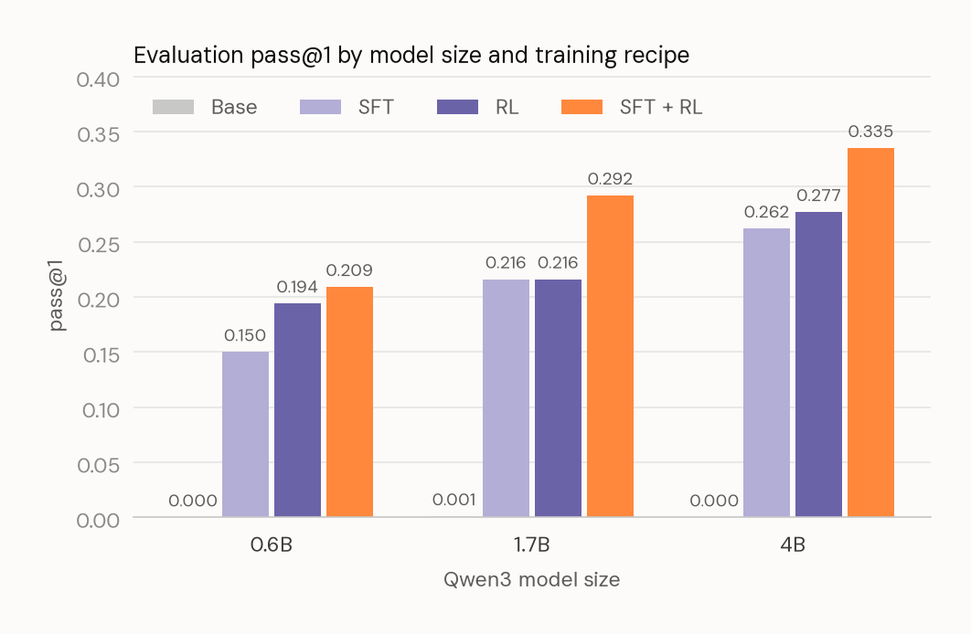
SFT + RL beats both SFT and RL alone at every size. Compared with pure RL, pass@1 improves by 0.015 at 0.6B, 0.076 at 1.7B and 0.058 at 4B. The interpretation we favor is that SFT fixes the format and provides a workable search policy, which puts the model in the band where GRPO groups have non-zero variance, so RL has something to reinforce.
With 242 evaluation questions, differences of a few hundredths are within noise, so the 0.015 gain at 0.6B should not be read as an improvement on its own. What matters more is the consistency: SFT + RL comes out ahead at all three model sizes.
The plot below puts the results from all three recipes together:
So far, we have only compared our models with each other. We know 4B with SFT + RL beats 4B with pure RL, but not whether 0.335 is close to the ceiling for this environment or a long way below it. The scorer is exact match against a gold answer, so a question that reads as answerable to us may still be near-impossible to score well on. To get an outside reference point, we ran a frontier model on the same harness.
Claude Haiku 4.5 on the same harness
We ran Claude Haiku 4.5 through the same environment and rubric, with extended thinking enabled and a 4,096-token thinking budget. The first run reused the Qwen prompt verbatim, which isolates the model as the only difference but gives Qwen an advantage: the prompt was written for it, and the SFT and RL runs were trained on it. Haiku scored 0.240 pass@1. Rewriting the prompt for Haiku (a turn-budget hint, few-shot examples and more detailed instructions on answer style) took it to 0.444.
| Setup | pass@1 | pass@2 | avg tool calls |
|---|---|---|---|
| Haiku 4.5, same prompt as the Qwen models | 0.240 | 0.317 | 6.23 |
| Haiku 4.5, prompt tuned for it | 0.444 | 0.522 | 5.46 |
A 0.20 jump from the prompt alone raises the question of what the same treatment does for our models. Adding the same information to the Qwen prompt improved performance only slightly (see the table below). At this point, our goal shifted from comparing recipes under equal conditions to getting the best possible performance out of the 4B model. Every run below therefore starts from the SFT checkpoint, the best starting point we have, and alongside the prompt, we made two other changes, both motivated by what the earlier runs had shown.
The first change was to the reward. The zero-advantage problem from earlier is a real cost here: a group whose rollouts all miss has no variance and no advantage, so dynamic sampling drops it, and at these pass rates that happens often. So we added a second term to the rubric, partial_credit, weighted 0.3 against exact_match's 1.0. It scores token overlap against the nearest gold answer using with , and is set to 1.0 whenever exact match succeeds. This separates "retrieved the right passage but mangled the span" from "wandered off entirely" inside an otherwise flat group. Reward curves are no longer comparable across this change, but pass@k is: the correct band scores 1.3, the incorrect band tops out at 0.3, and the 0.5 pass threshold sits in the gap between them.
The second change was to the corpus. Everything up to this point used MuSiQue's own validation split, 2,417 questions over 21.1k passages, which at 500 steps and 4 questions per update is about one pass through the data. MuSiQue's training split has 19,938 questions over 84.6k passages, a corpus four times as large with the same top- retrieval budget, so a gold paragraph has to outrank more competitors to reach the model. We trained on it for 2,400 steps.
Evaluation still uses the same 242 held-out questions against the 21.1k corpus throughout, which keeps the table below comparable to the ones above.
| Setup | pass@1 | pass@2 | avg tool calls |
|---|---|---|---|
| 4B, SFT + RL (from above) | 0.335 | 0.405 | 3.73 |
| 4B, SFT + RL + revised prompt | 0.347 | 0.437 | 3.53 |
| 4B, SFT + RL + revised prompt and reward | 0.395 | 0.470 | 3.55 |
| 4B, SFT + RL + revised prompt and reward + train split | 0.446 | 0.512 | 4.25 |
The last row is not a controlled comparison: it was trained on more data and for much longer, which alone could explain the improvement. It is simply our best configuration.
Haiku issues tool calls in parallel, while our Qwen models issue one per turn. With turns capped at 8, Haiku has much more room to explore within the same budget. As a final check, we gave the 4B model 16 turns at evaluation time to see what difference it makes.
| Setup | pass@1 | pass@2 | avg tool calls |
|---|---|---|---|
| 4B, SFT + RL + revised prompt and reward + train split, 16 turns at eval | 0.452 | 0.517 | 4.61 |
The extra turns help only marginally (0.452 versus 0.446), so the turn cap is not what holds the model back.
The pass@k metric tells us how often a model is right, but nothing about how it fails. To investigate the failure modes, we classified every evaluation rollout into one of four outcomes:
- Correct. Exact match against the gold answer or one of its aliases, after lowercasing and stripping non-alphanumeric characters. This is the same rule the reward uses, so this bucket matches pass@1 above.
- Near miss. An answer was given but missed exact match, while still overlapping substantially with a gold answer (unigram F1 ). Typical cases are an extra qualifier, such as "the city of Rotterdam" for "Rotterdam," or a partly correct multi-word entity.
- Wrong. An answer was emitted with less overlap than that.
- No answer. The final assistant message contains no
<<...>>block at all. These are mostly rollouts that hit the turn cap while still searching, plus a few that stopped responding. Some answered in an earlier turn and then kept calling tools; since only the last message is inspected, these count as no answer too.
The buckets are checked in that order, so every rollout lands in exactly one.
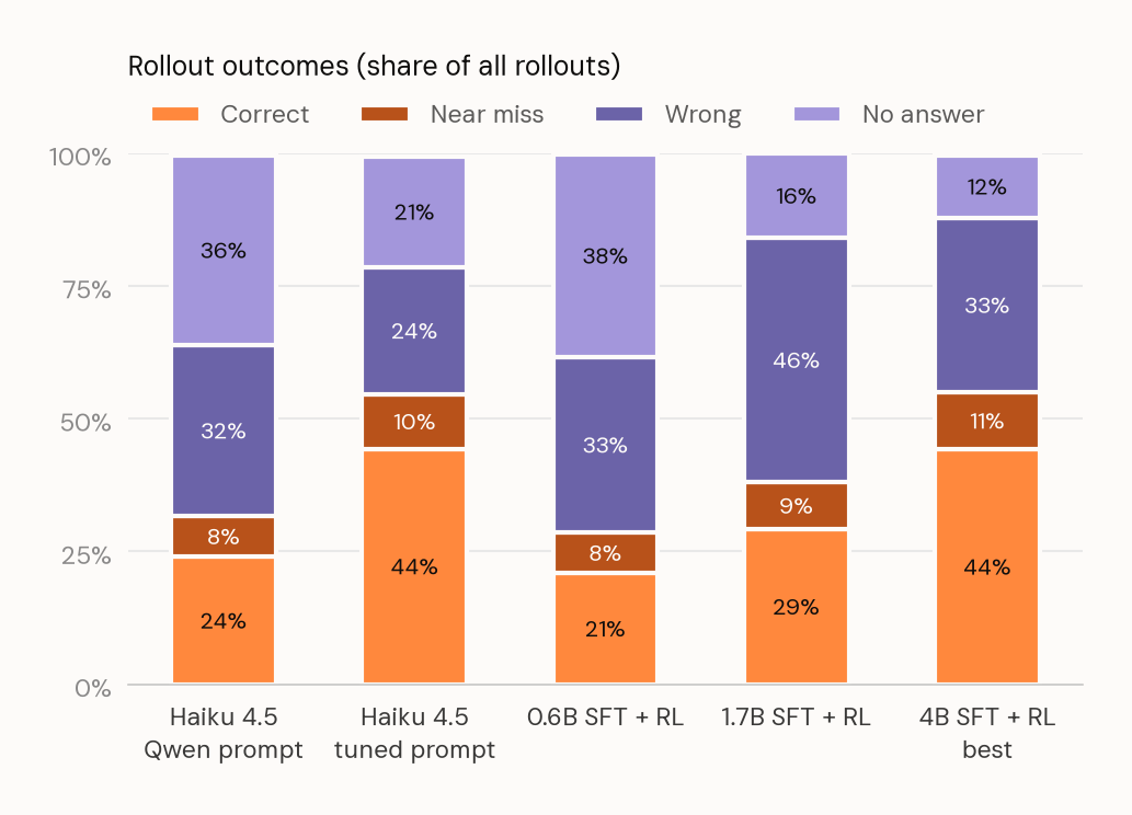
The failure modes differ by size. The 0.6B model spends its budget searching and gets stuck in long, circular reasoning, so it often runs out of turns before answering. The 1.7B model more often answers, but wrongly, and the traces suggest that the reasoning itself is sometimes the problem, especially with temporal relations. The 4B model usually finds the first passage but often loses the trail at the bridge entity, the entity revealed by one passage that the next search has to build on. The share of gold passages that show up in its search results drops from 92% at the first hop to 48% at the second. When it is wrong, it almost always commits to an answer anyway, and in about half these cases, it misread a passage it had already retrieved, typically by overlooking a date or succession qualifier. The near-miss band is a reminder that exact match and task success are not the same thing, and it is exactly this band that the partial_credit term rewards during training.
Stepping back from the failure modes to the headline result: our best 4B model (0.446) performs about as well as prompt-tuned Haiku (0.444). We set out to find how close a small self-hosted model trained with RL gets to a frontier-lab model, and on this task, the answer is very close. A 4B model running on our own hardware is in the same league as a frontier lab's small model.
Cost comparison
At the time of writing, Haiku 4.5 is billed at $1 per million input tokens and $5 per million output tokens, with thinking tokens charged at the output rate. The prompt-tuned eval came to $16.50 for 242 questions at 3 rollouts each. This is at list price without prompt caching. Haiku 4.5 only caches prompts of at least 4,096 tokens, and our prompt is well below that, so only the later turns of a rollout, once search results have accumulated in the conversation, would benefit. Caching would reduce the input portion of those turns, but not the output and thinking tokens, so the gap to self-hosting would narrow somewhat but remain large. We price our own runs at RunPod's on-demand rate for the card we train on, $0.53 per hour for an RTX A6000.
| Setup | Cost per 1,000 questions (one rollout each) |
|---|---|
| Haiku 4.5 | $23 |
| 4B SFT + RL, self-hosted | $0.61 (~37× cheaper) |
The self-hosted figure covers inference only: the full eval, 726 rollouts, takes 50 minutes on a single A6000. Training the LoRA adapters for the 4B recipe is a one-off cost of 305 GPU-hours, or $162 at the same rate (excluding the teacher rollouts used to build the SFT set). That is 1.5 hours of SFT on one card, followed by 152 hours of GRPO on two cards for the 2,400-step run. At $0.022 saved per question, the training pays for itself after roughly 7,300 questions, and every question after that costs about 37 times less than through the API.
The rental rate stands in for hardware we already own, which is the simplest way to give a number readers can check against their own setup; our own marginal cost is lower, since the cards are already paid for. The figure also counts only GPU time spent generating, not the server sitting idle between requests, so the gap narrows for a workload with a low duty cycle. That idle time is shareable, though: one base model can serve adapters for several tasks, so a deployment with modest volume per task can spread the same GPU across all of them instead of paying for a card per task.
Conclusion
The narrow task was easy. A 0.6B model saturated it after a few hours of training on two A6000s, and beyond that point the environment, not the model, was the limit.
The open-ended task was harder, and there the recipe mattered roughly as much as model size. A 1.7B model trained with SFT and then RL matched a 4B model trained with RL alone. Our best 4B run ended up close to prompt-tuned Haiku 4.5 on the same harness, at a small fraction of the cost per question.
A few practical lessons carry over to other tasks. Check the base model first: if it never succeeds, GRPO has nothing to learn from, but near-zero is often a formatting problem rather than a capability one. A small SFT set from a stronger teacher fixes that cheaply, as long as you filter out trajectories that reach the right answer without doing the task. Partial credit in the reward gives flat groups something to learn from. Finally, none of this required much compute. Our best run took about 300 GPU-hours on two RTX A6000s.
A frontier API is the easiest place to start, but it is not the only option. On our retrieval task, a 4B model served from a single card of our own got roughly as far as the API model. If you can write a verifier for your task, it is worth testing whether a small model can do the same. A self-hosted model also stays under your control. Nobody deprecates it, it only changes when you change it, and the data never leaves your hardware. What you give up is generality: the API model can do almost anything, while yours does one task. But most production agents do one thing, over and over, and for those, a small model trained for that task may be all you need.
Notes
[1] Sampling more rollouts per question is a way to check whether correct trajectories exist in the model's distribution at all, rather than whether they are likely. Yue et al. [2025] use pass@ at large in this way to argue that RLVR at small works by concentrating probability mass onto trajectories the base model already produces occasionally, which is why a non-zero pass@16 counts as evidence that there is something to train on, even when pass@1 rounds to zero. Their stronger claim, that base models overtake RL-trained ones once is large and RLVR therefore cannot expand the reasoning boundary, is contested: Liu et al. [2025, ProRL] report the opposite under prolonged training with KL control and reference-policy resets, and Yuan et al. [2026] argue that the high- decline is an artifact of overtraining rather than evidence about capability. Nothing here depends on that dispute. The weaker claim, that gains at small come from reweighting trajectories already present in the base distribution, is not in question.
References (14)
Williams, Simple Statistical Gradient-Following Algorithms for Connectionist Reinforcement Learning, 1992.
doi:10.1007/BF00992696Schulman et al., Proximal Policy Optimization Algorithms, 2017.
arXiv:1707.06347Shao et al., DeepSeekMath: Pushing the Limits of Mathematical Reasoning in Open Language Models (GRPO), 2024.
arXiv:2402.03300Prime Intellect, prime-rl.
github.com/PrimeIntellect-ai/prime-rlPrime Intellect, verifiers.
github.com/PrimeIntellect-ai/verifiersYu et al., DAPO: An Open-Source LLM Reinforcement Learning System at Scale, 2025.
arXiv:2503.14476Liu et al., Understanding R1-Zero-Like Training: A Critical Perspective (Dr. GRPO), 2025.
arXiv:2503.20783Prime Intellect, INTELLECT-2: A Reasoning Model Trained Through Globally Decentralized Reinforcement Learning, 2025.
arXiv:2505.07291Jin et al., Search-R1: Training LLMs to Reason and Leverage Search Engines with Reinforcement Learning, 2025.
arXiv:2503.09516Shrivastava et al., ECHO: Terminal Agents Learn World Models for Free, 2026.
arXiv:2605.24517Trivedi et al., MuSiQue: Multihop Questions via Single-hop Question Composition, 2022.
arXiv:2108.00573Yuan et al., Understanding Diversity Collapse in RLVR via the Lens of Overtraining, 2026.
arXiv:2606.15455Yue et al., Does Reinforcement Learning Really Incentivize Reasoning Capacity in LLMs Beyond the Base Model?, 2025.
arXiv:2504.13837Liu et al., ProRL: Prolonged Reinforcement Learning Expands Reasoning Boundaries in Large Language Models, 2025.
arXiv:2505.24864
Learn more