Branching Flows: variable-length flow matching

Introduction

Diffusion and flow matching have taken over generative modelling for anything that is not text. They produce images, video, molecules and protein structures by transporting a simple noise distribution onto a data distribution along a learned velocity field. The machinery is elegant, the samplers are fast, and the results speak for themselves.

They also share a limitation that is easy to miss, because it is built into the mathematics rather than bolted on afterwards. A flow moves a fixed set of elements. The same points that start as noise at $t = 0$ arrive as data at $t = 1$. Nothing is ever created, and nothing is ever destroyed. So the number of elements in the output has to be decided before the model starts running: how many atoms in the molecule, how many residues in the protein, how many tokens in the sequence.

For protein design that is a genuine problem. If you are designing a binder against a target, the number of residues in the binder is one of the things you wanted the model to tell you. In practice it gets handled by sweeping over candidate lengths, sampling many designs at each one, and filtering afterwards.

Branching Flows removes the constraint. Elements evolve over forests of binary trees: each one can split into two, or die off, at rates the model learns alongside the ordinary velocity field. The number of elements becomes an output of the generative process rather than an input to it. This post walks through how it works, starting from flow matching itself.

Flow matching

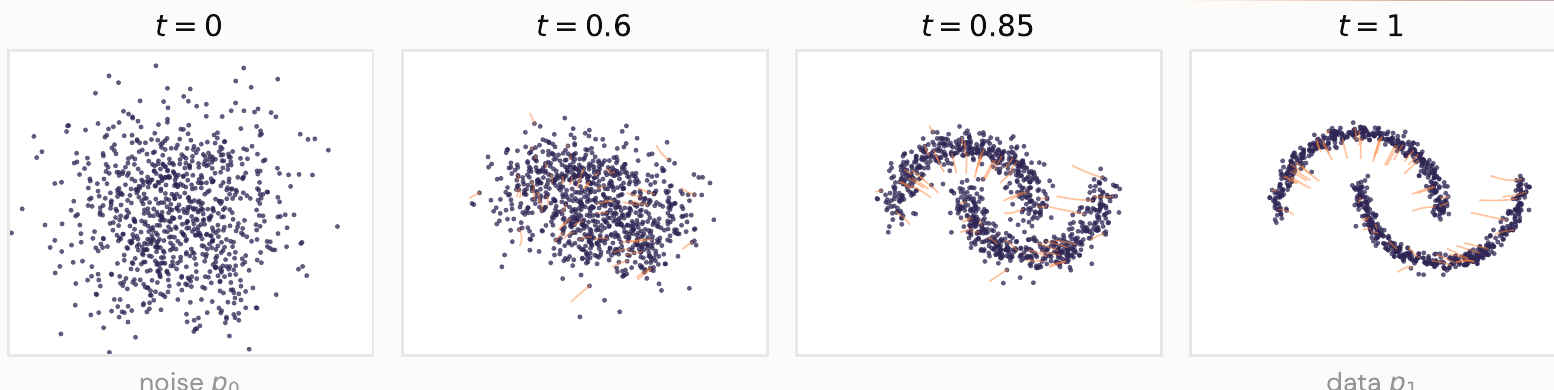
The setup is a transport problem. We have a simple distribution $p_0$ that we can sample from, usually $\mathcal{N}(0, I)$, and a data distribution $p_1$ that we cannot. We want a map that carries one onto the other, and we want to learn it from samples alone.

Flow matching does this with a time-dependent velocity field. Each sample follows a smooth path, governed by an ordinary differential equation:

The flow $\psi_t$ pushes the base distribution forward, $p_t = [\psi_t]_\# \, p_0$, and we want the result to be $p_1$ when $t = 1$. The density and the velocity are tied together by the continuity equation:

Time here runs from noise at $t = 0$ to data at $t = 1$. In much of the diffusion literature the convention runs the other way, which is worth keeping in mind when comparing papers.

The obvious objective is to regress a network onto the true velocity field:

We cannot optimise this directly. We know neither $u_t$ nor the probability path $p_t$ it induces, and if we knew $u_t$ there would be nothing left to learn.

The conditional flow matching trick

The way out, from Lipman and colleagues, is to specify the path ourselves instead of inferring it from the field. Pick a path conditioned on both endpoints, for example a straight line:

The conditional velocity $u_t(x_t | x_0, x_1)$ is just the derivative of that line. Sampling $p_t$ is now easy, and it is hierarchical: draw $x_0$ from the noise and $x_1$ from the data, then take a point on the line between them. The choice of the endpoint conditional path induces:

Training then regresses against the conditional velocity, and the key result is that this has the same gradient as the intractable objective:

This pattern is worth internalising, because Branching Flows reuses it exactly: choose a conditional process you can write down, take an expectation to recover the marginal object, and train against the conditional target.

Sampling

Once $u^\theta_t$ is trained, generating a sample is just solving an ODE. Draw $x_0 \sim p_0$, then integrate $\dot{x} = u^\theta_t(x)$ from $t = 0$ to $t = 1$, in practice with Euler steps $x \leftarrow x + \Delta t\, u^\theta_t(x)$.

Discrete flow matching

The same recipe works when the state is categorical, with a continuous-time Markov chain in place of an ODE. Rather than drifting along a velocity field, the state jumps:

The rate matrix $Q_t$ has $Q_t(y \mid x) \ge 0$ for $y \ne x$ and rows summing to zero, and the density evolves by the Kolmogorov forward equation, $\partial_t\, p_t(y) = \sum_x Q_t(y \mid x)\, p_t(x)$.

Structurally nothing has changed. You still pick conditional paths and learn the marginal object by taking an expectation: a velocity in the continuous case, rates in the discrete one. Sampling becomes a sequence of jumps, where at each step you move to $y$ with probability $Q^\theta_t(y \mid x)\, \Delta t.$

Use cases of Flow Matching

Here are some examples of how flow matching models are used today.

1. Image generation models. We transport a noisy image to a clean image from the data distribution. This uses a continuous state space: each pixel holds continuous values (think one value for each RGB channel).

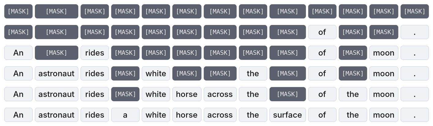
2. Diffusion language models. We transport masked tokens to text. This uses a discrete state space of tokens.

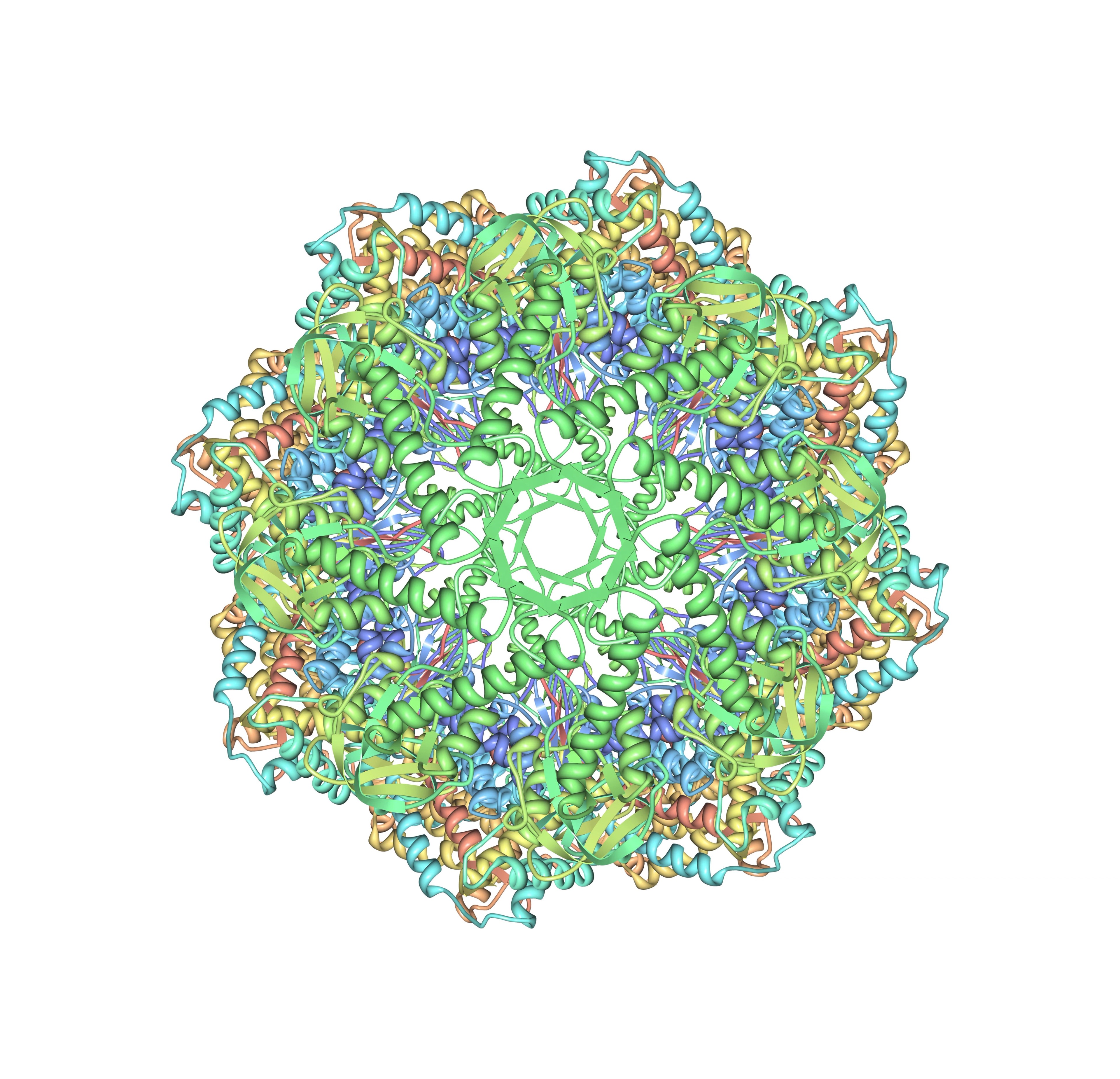
3. Protein design. We generate a new protein. This combines two state spaces: the discrete amino acid identities and the continuous residue positions in Euclidean space (sometimes extended with residue orientations on a manifold, such as SO(3)).

Note that in all three of these applications, the state space was fixed and known before the flow began. In the image example, we already knew the number of pixels; in the language model, we had already laid out a fixed number of masked tokens; and in the protein design model, we started with a point cloud of a fixed number of amino acid residues. No change in dimensionality occurred during the flow. We had to specify it beforehand! This is an important limitation of flow matching.

The variable-length problem

Flow matching works on a fixed state space: $x_0$ and $x_1$ have the same dimensions. That’s fine for applications like image generation, where we usually know the pixel dimensions of the image we want to create beforehand. In protein design, however, it’s more of an issue. We might not know a priori how long a binder should be; ideally the model itself should decide the length at sampling time. This is what we mean by the variable-length problem. The usual approach in protein design is still to train a fixed-length model and sweep across different lengths, which is somewhat ad hoc. Letting the model decide the length itself is the main idea behind Branching Flows.

Another way to see the variable-length problem is through infilling. Suppose you have a prefix A and a suffix B, and you need to generate what goes between them. This is a generative task conditioned on the flanking regions, and plenty of models can already do it, as long as we specify the length beforehand. Masked transformers fill in [MASK] positions; diffusion and flow models denoise the span. Both need the number of missing positions up front, and in infilling that number is not a minor detail. Consider a sentence with a gap of unknown size:

The main takeaway is that the length decides which meanings are reachable at all. Choosing a length is not a technical detail; it is part of deciding what the output says. Sweeping over lengths by hand is therefore an ad hoc workaround for a choice that should ideally be made by the model itself. The same is true in protein design: the length of a binder is itself a design variable with functional consequences.

Branching Flows

Branching Flows is a framework that extends flow matching to variable-length generation, where the model itself decides the length. Here’s an example of what that looks like:

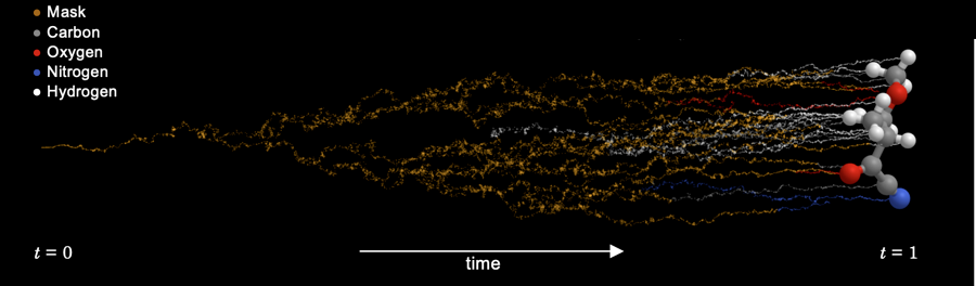
Rather than inserting new elements at arbitrary positions, which would force the model to learn a distribution over where each one belongs, Branching Flows grows the sequence by splitting: an existing element duplicates in place, and the base process then moves the two copies apart. Elements can also be deleted, and both splits and deletions happen at rates the model learns. Because a new element always starts exactly where its parent was, the construction works for discrete, continuous and manifold states, or any mix of them. That matters for molecules and proteins, where each element has both a position and a label (an atom or amino acid type).

Everything evolves together. The learned field $u^θ_t$ reads the whole state and outputs velocities for the atom positions, rates for the discrete atom types, and on top of that the split and deletion rates. This means the model can correct itself as it goes: if it needs more elements, one splits into two, and if an atom is badly placed, it can be deleted. Length becomes an output of the model, not an input.

How Branching Flows is trained

As covered earlier, flow matching trains on simple endpoint-conditional paths rather than the intractable marginal one. Branching Flows does the same, but here $x_0$ and $x_1$ have different lengths, so the path must also decide which elements split, which are deleted, and when. The authors handle this by conditioning on a richer latent variable than just the endpoints.

1. Sample Z

Alongside a data point $x_1 \sim q,$ we sample $z = (x_1^{+\emptyset}, x_0, \mathcal{T}, \mathcal{A})$:

• $x_0$: the initial noise elements, often just a few ones.
• $x_1^{+\emptyset}$: the data with extra “to-be-deleted” copies inserted.
• $\mathcal{T}$: a forest of binary trees linking each root in $x_0$ to the leaves of $x_1^{+\emptyset}$, built by repeatedly merging random adjacent pairs, which preserves the sequence order.
• $\mathcal{A}$: an anchor for every node. A surviving leaf’s anchor is its data element, and each internal anchor is a weighted average of its children’s anchors (a mask token for discrete components).

2. Conditional paths

Given $z$, each element follows the base process towards the anchor of the node ahead of it. It splits in place at a rate proportional to its number of remaining splits, after which each copy heads for its own child’s anchor. Elements on branches ending in a to-be-deleted leaf can also be deleted. Both rates diverge as $t → 1$, so every scheduled event has happened by the end, and the path terminates exactly at $x_1$. The figure below shows one such conditional path.

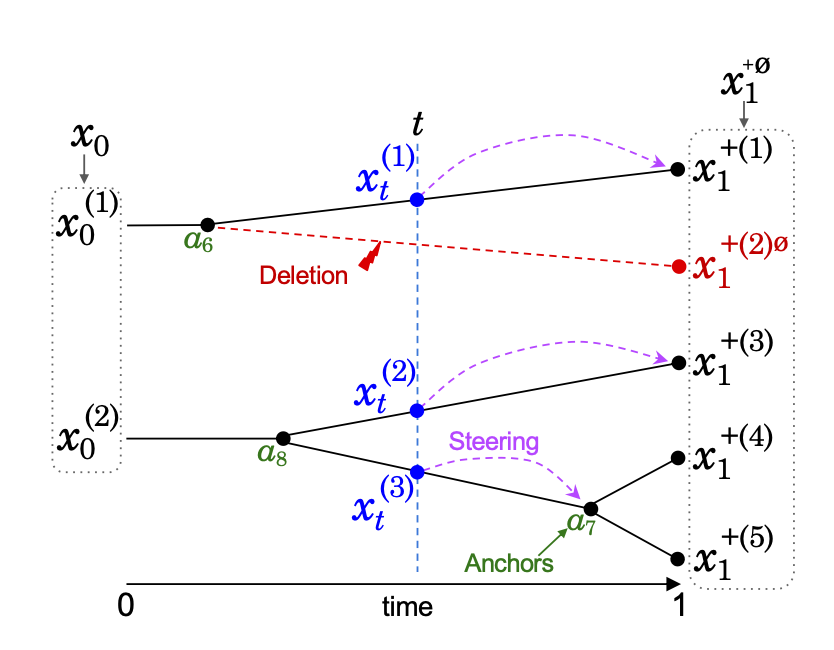
Between events, nothing unusual happens: each element does ordinary flow matching towards the next anchor, exactly as if that anchor were $x_1$. The branching sits on top of whatever base process you choose, whether that’s a plain ODE, an Ornstein–Uhlenbeck process, a Riemannian flow or discrete flow matching. Branching Flows extends the flow matching design space rather than replacing it.

Because $z$ is fixed, everything in the figure is known in advance: how many more times each element will split, whether it will be deleted, and which anchor it is heading for. The model never gets to see $z$, so it has to learn to predict these quantities from the current state alone. That is exactly what it is trained to do.

3. Training targets and loss

For each element at time $t$, the model predicts its expected number of remaining splits, its probability of eventually being deleted, and the usual base-process output. The loss is a sum of Bregman divergences: Poisson-style for splits, cross-entropy for deletions, and the base-process loss (for example, squared error or discrete flow matching). As in ordinary flow matching, training on these conditional targets is enough for the model to learn the right overall process. At sampling time, it only needs the current state $x_t$, not $z$.

What Branching Flows can do

Now let's see the model in practice. We demonstrate four tasks:

1. Unconditional protein design — we start from a few masked amino acids and let the model run.
2. Binder design — we fix a target protein and design a second protein that binds to it.
3. Infix sampling — a protein complex is missing a section, which we fill back in.
4. Unconditional small-molecule generation (QM9) — we start from a single masked atom and generate a molecule.

We show one sampling video each. We begin with an element drawn from the noise distribution and integrate it according to our base process, together with the splits and deletions, which is what the videos below show. In each video, the left panel shows the flow (the sample being integrated), and the right panel shows the endpoint prediction: the trained model works by predicting the endpoint and then rescaling it to a velocity.

Plug and Play

For anyone who already has a trained flow matching model, the most immediately useful part of the paper is how easily Branching Flows can be added to it.

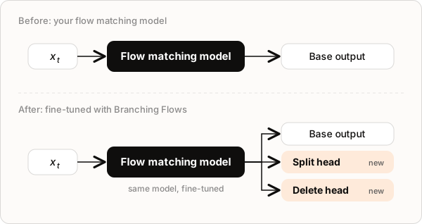
As Figure 4 shows, no new architecture is needed. You take any pretrained fixed-length flow matching model and add two heads, one for splits and one for deletions. Then you fine-tune the whole network with Branching Flows and add a split-and-delete step to the sampling loop. The authors report that three days on a single NVIDIA RTX 6000 Ada was enough, and they did this both with their own ChainStorm model and with NVIDIA’s La Proteina.

Practical guidance: three choices helped the authors: using a stochastic base process with learned drift and fixed noise, placing most splits early so new elements had time to settle, and predicting each element’s endpoint rather than its drift directly, which proved more stable. The authors’ open-source code is available on https://github.com/MurrellGroup/BranchingFlows.jl .

Closing thoughts

Branching Flows extends flow matching by making the number of elements part of the generative process itself. This opens the door to variable-length generation, including infilling problems where even the number of missing elements is unknown. Existing models don’t need to be rebuilt from scratch: adding split and deletion heads and fine-tuning is enough to bring them over. Taken together, this meaningfully expands what we can ask flow-based models to generate.